The starting point was a product problem, not an equation. ItoFlow users do not ask only, "What was my volatility?" They ask why the portfolio is risky, whether the risk is intentional, how it differs from the benchmark, and what a rebalance would actually change. A returns-covariance matrix can estimate total risk, but it rarely explains the portfolio in a language a user can act on.
We therefore built an in-house factor risk model. The goal was not to recreate every feature of a commercial institutional model. The goal was to build a disciplined, transparent model that works for the portfolios people actually hold: global equities, India and UK names, US mega-caps, ETFs, funds, gold, Treasuries, and cash-like instruments.
A risk factor is a common source of return variation. If global equities sell off, many stocks move together because they share market beta. If oil prices jump, energy producers and airlines may move for related but opposite reasons. If investors rotate out of expensive growth stocks, a portfolio tilted toward long-duration technology companies can lose money even when no individual company-specific news has arrived.
That is the basic insight behind factor risk models. A portfolio of AAPL, MSFT, NVDA, QQQ, and XLK may look diversified by ticker count, but much of its risk is likely one bundle: global equity beta, US equity exposure, information technology, growth or momentum, and some single-name concentration. Conversely, two portfolios with the same number of holdings can have completely different risk: one may be a concentrated bet on India financials, another a blend of US equities, gold, Treasuries, and cash-like funds.
A returns-covariance matrix can say which holdings moved together. A factor model tries to explain why they move together in economically named buckets. That changes the portfolio conversation from "volatility is 14%" to "44% of forecast risk is broad equity beta, 26% is single-stock risk, and the rest comes from country, style, sector, and cross-asset effects."
That matters because the same decomposition improves both investor oversight and portfolio construction. A human monitoring a portfolio needs to know whether risk is intentional: "we chose UK equity risk" is different from "we accidentally built a UK factor bet." A portfolio process also benefits from the same decomposition because optimization, rebalancing, and benchmark-relative decisions are all better when the objective is expressed in risk drivers rather than ticker counts.
A risk language for portfolios. A useful factor model lets investors and portfolio systems ask practical questions: which risks dominate the book, which ones diversify it, which ones are benchmark-relative active bets, and which ones are merely company-specific concentration?
What are risk factors?
A risk factor is a reason holdings move together. A factor model asks: if the portfolio moves tomorrow, is it because global equities moved, because India sold off, because technology stocks rotated lower, because small caps underperformed, or because one company had bad news? Some factors appear in almost every equity portfolio; others matter only when the portfolio has a particular country, sector, style, ETF, or single-name concentration.
| Risk driver | What it measures | How to read it in a portfolio |
|---|---|---|
| Global stock-market beta | Sensitivity to broad equity markets moving together. | Usually the largest driver in a long-only equity portfolio. A high share means the portfolio is mainly being paid, or punished, for owning equities. |
| Country equity markets | Exposure to the equity market of the company's primary country, or a fractional country mix for equity funds with holdings data. | Useful for seeing whether a portfolio is really a US, UK, India, Europe, or global equity bet. |
| GICS sectors | Exposure to economically related industries such as information technology, financials, health care, energy, utilities, or real estate. | Reveals sector concentration that ticker count hides. Ten stocks can still be one technology bet. |
| Size | Whether the portfolio tilts toward smaller or larger companies after normalizing across the investable universe. | Small-cap and mega-cap portfolios can behave differently even if their sector weights look similar. |
| Value and growth | Whether holdings look cheap relative to fundamentals, or have stronger historical growth characteristics. | Captures the risk of style rotations: cheap stocks rallying, expensive growth stocks selling off, or the reverse. |
| Momentum | Recent price trend, usually measured over an intermediate window rather than yesterday's move. | Shows whether the portfolio depends on recent winners continuing to win. |
| Quality | Profitability, margins, leverage, and balance-sheet strength after sign alignment and standardization. | Separates portfolios tilted toward durable, profitable businesses from those taking more balance-sheet risk. |
| Volatility and liquidity | Historical price variability and trading depth or turnover. | Highlights exposure to unstable prices or less-traded stocks, which can matter most during stress. |
| Company-specific risk | The part of risk left after market, country, sector, and style effects are explained. | Important for concentrated portfolios. It is the risk of individual holdings surprising the portfolio. |
| Cross-asset covariance | How equity risks move with assets outside the equity factor model, such as gold, Treasury funds, bond ETFs, or cash-like instruments. | Prevents a mixed portfolio from pretending equities, bonds, gold, and cash-like funds are unrelated. |
The build process came down to one discipline: make \(X F X^\top + D\) true for real portfolios, not toy portfolios. That meant designing for global stocks, ETFs, funds, cash-like instruments, different trading calendars, incomplete security data, benchmark-relative views, and explanations compact enough for a person to actually read.
Step 1: start with the object we want to forecast
For portfolio weights \(w\), the target object is total portfolio variance. That mean-variance object goes back to Markowitz's formulation of portfolio selection, where covariance between assets is central rather than incidental.[1]
A returns-covariance model estimates \(\Sigma\) directly from historical asset returns. That is often a very strong baseline. It works for common stocks, ETFs, bond funds, gold funds, and anything else with enough return history. But it is also a black box. It does not tell the user whether risk comes from market beta, UK equity exposure, technology, small-cap stocks, a momentum tilt, or one concentrated name.
A factor model decomposes the asset covariance matrix into systematic and specific components. That idea sits between academic asset-pricing factors, such as the market, size, and value factors studied by Fama and French, and practitioner risk models such as MSCI Barra, which focus on forecasting and attributing portfolio risk.[2][3]
Here \(X_E\) is the exposure matrix for equity-like instruments, \(F_E\) is the factor covariance matrix, and \(D_E\) is diagonal specific variance. The word "diagonal" matters: in this baseline formulation, residual shocks are treated as security-specific after common exposures are removed. That is not a claim that issuer-level or dual-listing residual covariance never exists. It is a disciplined starting point.

The left matrix is factor covariance. The right matrix is the resulting asset covariance after applying loadings and specific risk. Portfolio variance is \(b' F b + w' D w\), where \(b = X' w\).
Step 2: separate exposure from risk
A common mistake is to stop once factor loadings exist. Loadings answer the exposure question: "What is this portfolio sensitive to?" Risk needs the covariance of those factors. A portfolio can have a large positive exposure to a factor that is currently diversifying other exposures, or a small exposure to a factor with high volatility and high covariance with the rest of the book.
The portfolio factor exposure is:
The systematic variance is:
The specific variance is:
And total model variance is:
That is the quantity investors intuitively care about, but it is not always the clearest way to present risk. The useful decomposition separates variance contribution, marginal contribution to volatility, and percentage share of total forecast variance. For factor \(k\):
Company-specific risk has an analogous contribution: security \(i\) contributes \(w_i^2 d_i\) to variance, and the portfolio-level company-specific share is \(\sum_i w_i^2 d_i / \sigma_p^2\).
This is why the chart should say "what drives portfolio risk", not merely "factor exposures". The former is a decomposition of forecast volatility. The latter is just the position of the portfolio in factor space.

Risk contribution is sorted by importance. Negative bars are possible because covariance can make one factor hedge another. That is not an error; it is a natural result of covariance.
Step 3: build the exposure matrix
The equity model starts with a matrix \(X\), one row per symbol and one column per factor. The columns are deliberately a mix of deterministic classification factors and continuous style descriptors. For industry classification, the model uses the Global Industry Classification Standard as the economically legible taxonomy rather than inventing sector labels from tickers or exchange suffixes.[4]
| Factor family | Loading construction | Why it matters |
|---|---|---|
| Global stock-market beta | Common stocks carry broad equity-market exposure. This factor captures the portion of risk shared with global stock markets. | Most long equity portfolios are dominated by the broad equity market. |
| Country equity market | Common stocks receive one primary country exposure. Equity ETFs may receive fractional country exposure from their underlying holdings. | Global portfolios need to distinguish US, UK, India, EU, and other equity-market risks without inferring country from ticker suffixes. |
| GICS sector | Common stocks receive one GICS sector exposure. Equity ETF sector exposure comes from holdings look-through when available. | Sector is more stable for the current investable universe than sparse industry or sub-industry factors. |
| Style | Size, value, growth, momentum, quality, volatility, and liquidity are standardized descriptors computed before the return fit. | Styles capture common ways portfolios differ even when their sectors look similar. |
| Specific risk | Residual variance after fitting common factors. High-leverage or short-history names are treated conservatively when the estimate is unreliable. | A concentrated portfolio can have high risk even after market, country, sector, and style effects are explained. |

The blank rows for GLD and SGOV are intentional. They are not common-stock equity exposures, so they do not receive country, sector, or equity-style loadings in this matrix. Their risk still counts: gold and short-Treasury ETFs are measured from their own return histories and then combined with the equity model in the full portfolio covariance. A zero here means "not an equity factor exposure," not "missing data" or "zero risk."
Why deterministic country and sector exposures are not optional
Country and sector are not estimated by regressing each stock on country or sector proxies. For a common stock, they are characteristics. A US software company should have a US country loading of \(1.0\) and a software or technology sector loading of \(1.0\), subject to the model's chosen taxonomy. The regression then estimates the daily return to those common characteristics across the cross-section.
That distinction is important. If country and sector were estimated as rolling time-series betas, the model could quietly explain away a missing classification problem as a low beta. Deterministic classification makes data-quality problems visible. If reliable classification data is unavailable, the model should disclose lower confidence rather than infer country or sector from a ticker suffix.
How styles enter the model
Style factors are different. Size, value, growth, momentum, quality, volatility, and liquidity are continuous descriptors. The key product decision is to name them in investor language. "Liquidity" should read like "less-traded stock risk". "Size" should say whether positive means small-cap or large-cap tilt. "Global Equity Market" should read like "global stock-market beta". The math can be institutional; the labels cannot require institutional memory.
Style construction is a cross-sectional measurement problem. Let \(u_{i,m}\) be raw descriptor \(m\) for security \(i\): book-to-price, earnings yield, trailing momentum, realized volatility, market capitalization, dollar trading volume, and so on. Raw descriptors are not comparable. A 12-month return, a leverage ratio, and a market capitalization live on different scales and have different outlier behavior.
The first step is therefore to winsorize each raw descriptor inside the model universe:
Here \(q_m(\alpha)\) and \(q_m(1-\alpha)\) are lower and upper cross-sectional quantiles for descriptor \(m\). The point is not to erase outliers; it is to stop one stale fundamental, split artifact, or extreme ratio from defining the factor.
Each winsorized descriptor is then standardized cross-sectionally:
A composite style loading is built from standardized subdescriptors, not from raw ratios:
\(M_k\) is the descriptor set for style \(k\), \(a_{k,m}\) is the sign and weight of each subdescriptor, and \(\mathbf{1}_{i,m}\) records whether security \(i\) actually has descriptor \(m\). Re-standardizing \(g_{i,k}\) gives the final loading \(x_{i,k}\): roughly, how many cross-sectional standard deviations the security sits away from the average stock on that style.
| Style | Example raw measures | Sign convention |
|---|---|---|
| Size | Market capitalization | Positive can be defined as smaller-cap tilt by using \(-\log(\text{market cap})\). |
| Value | Book-to-price, earnings yield, sales-to-price | Positive means cheaper relative to accounting fundamentals. |
| Growth | Sales growth, earnings growth, asset growth | Positive means stronger historical growth characteristics. |
| Momentum | Trailing price return, usually excluding the most recent month | Positive means stronger recent price trend. |
| Quality | Return on equity, gross margin, leverage | Positive means more profitable and less balance-sheet-stressed after sign alignment. |
| Liquidity | Dollar trading volume, turnover, trading capacity | Positive should match the label: either more liquid or less liquid, but never ambiguous. |
As a concrete example, suppose a stock has value subdescriptor z-scores of \(+1.4\) for book-to-price and \(+0.8\) for earnings yield, but sales-to-price is unavailable. With equal weights, the provisional value score is \((1.4 + 0.8)/2 = 1.1\), and descriptor coverage is \(2/3\). The missing third input is not filled with zero. The model records the lower coverage, then re-standardizes the composite against the rest of the universe before using it in \(X\).
That coverage line is not cosmetic. Missing fundamentals are not the same as average exposure. If a security lacks the data required for a style descriptor, the model should mark the descriptor as incomplete rather than silently treating the security as average.
Step 4: estimate factor returns
Once \(X_t\) exists, daily factor returns are estimated cross-sectionally:
Here \(r_t\) is the vector of symbol returns for date \(t\), \(f_t\) is the vector of factor returns, and \(e_t\) is the residual return vector. This is not a time-series beta regression per stock. It is a daily cross-sectional fit: on each date, explain the cross-section of stock returns with the current exposure matrix.
A global model has to handle global calendars. A US stock may not trade on July 4. An Indian stock may trade that day. A UK stock has a different holiday calendar. The model computes per-symbol returns on each symbol's own non-null price calendar, then aligns the return panel. This avoids manufacturing zero returns or false jumps from market holidays.
Currency matters. Returns are dimensionless, but the currency basis still matters. If a UK stock is priced in GBP and portfolio risk is reported in USD, the USD return includes the local equity return and the GBP/USD exchange-rate move between \(t_{\text{prev}}\) and \(t\):
\[ 1 + r^{USD}_{i,t} = (1 + r^{local}_{i,t})(1 + r^{FX}_{c(i),t}) \]
For small daily moves, \(r^{USD}_{i,t} \approx r^{local}_{i,t} + r^{FX}_{c(i),t}\). Currency should come from reliable instrument data. If currency information is missing, it is a data-quality issue, not permission to assume USD.
Step 5: make classification factors identifiable
A full market intercept plus complete country dummies plus complete sector dummies is not identified without constraints. If every common stock has market loading \(1.0\), one country loading, and one sector loading, there are linear dependencies. The model must decide what country and sector returns mean.
ItoFlow treats country and sector effects as relative effects by imposing weighted sum-to-zero constraints:
Rather than estimating covariance in the full redundant factor space, the model changes coordinates. Let \(Z\) be an orthonormal basis for the nullspace of \(C\):
Then covariance shrinkage happens in the reduced coordinate system:
This detail is easy to miss and expensive to get wrong. If we shrink directly toward a diagonal target in the full constrained factor space, we can create variance in directions the factor-return regression declared non-identifiable. Shrinking in the identified subspace keeps the covariance matrix consistent with the constraints. Shrinkage itself is not cosmetic; large covariance matrices are famously unstable without conditioning.[5]

The reduced covariance \(G\) is estimated in the nullspace coordinates. Mapping back with \(F = ZGZ'\) preserves the classification constraints.
Step 6: estimate company-specific risk
Specific risk comes from residual history. For symbol \(i\), the residual series is:
The naive residual variance is:
But a practical model needs more than the naive estimate. A sparse country or sector factor can partially fit one high-leverage stock and push its residual risk too low. Short-history names need lower confidence. Extremely small residual variances need floors. Peer shrinkage and leverage diagnostics are not bells and whistles; they prevent a factor model from treating the least reliable estimates as the safest assets.
Step 7: extend the model to ETFs and mixed assets
ETF wrappers are not exposures. A gold ETF is not a gold-mining equity. A Treasury ETF is not a bank stock. A broad equity ETF is not one issuer's sector classification. For mixed portfolios, the model follows a simple rule:
Use the most economically faithful risk representation available: factor exposure for covered equities, holdings look-through for equity ETFs, and return history for assets outside the equity factor model. Do not force non-equity assets into equity factors.
For an equity ETF with holdings data, look-through creates synthetic factor loadings:
And synthetic specific variance can be approximated by constituent specific risk:
If an ETF is represented by a proxy or partial look-through rather than complete holdings, the unexplained tracking error belongs in specific risk rather than being silently ignored.
If look-through is missing or only partially mapped, the portfolio still needs a total covariance estimate. A mixed-asset covariance matrix keeps factor-covered equities in the factor block and keeps other instruments in a return-history block:
The cross terms \(C_{E,A}\) and \(C_{A,E}\) are essential. Assuming equities, bonds, gold, and cash-like funds have zero covariance is usually worse than admitting that some symbols need return-based treatment.

The teal outline marks the equity block, where covered stocks and equity ETFs use factor-modeled risk. The gold outline marks instruments whose risk is measured from their own return history. The off-diagonal cells preserve cross-asset covariance, such as equity exposure versus gold or Treasury funds.
Step 8: turn risk estimates into explanations
A risk model only becomes useful when it can be reduced to a few stable questions: what drives total risk, what differs from the benchmark, how much is company-specific, and which holdings explain each driver?
The first view should therefore be compact by default: top risk drivers, company-specific risk as its own line, benchmark-relative view, and a clear statement of measured coverage. The advanced view can expose the mathematics, but the first screen should answer the portfolio question in plain language.

The same risk calculation should explain portfolio risk, benchmark-relative risk, and rebalancing trade-offs.
Making the model understandable
The useful view is the one that answers recognizable portfolio questions: how much risk comes from broad equity markets, how much from a country or sector tilt, how much from individual names, and which exposures offset one another. The calculation stays quantitative; the labels should make the risk drivers readable.
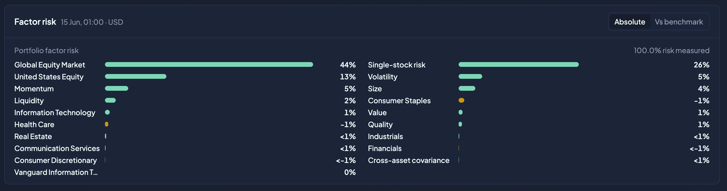
An ItoFlow portfolio risk view. The largest drivers appear first, with single-stock risk, benchmark-relative comparison, and measured coverage in one scannable panel. Values shown are illustrative and may differ from current estimates.
A concise view should show the top contributors first, sorted largest to smallest, with company-specific risk as its own row and a compact "other measured risk" row. A detailed view can explain which holdings contribute to each driver. Benchmark-relative analysis answers a different question: "What risks make this portfolio different from its benchmark?"
Step 9: calibrate the model to forecast risk
A factor model earns trust by forecasting risk, not by producing a plausible-looking decomposition. ItoFlow calibrates the model against realized portfolio volatility and against strong return-covariance baselines. That is the standard volatility models should be held to: their central job is forecasting future volatility, not merely fitting the past.[6]
The first rule is point-in-time discipline. A historical risk estimate should use only information that would have been available on or before the portfolio date:
That means no use of current-period loadings, current-period fundamentals, or current-period ETF holdings as if they were known in the past. Price-derived descriptors such as momentum, volatility, and liquidity can be reconstructed historically. Fundamental descriptors require explicit data provenance, and when historical fundamentals are incomplete the limitation should be visible rather than hidden inside an average exposure.
The calibration work has four layers:
| Validation layer | What is tested | Why it matters |
|---|---|---|
| Forecast calibration | Predicted variance versus future realized variance across rolling windows. | The model should get the scale of risk right, not only the direction of the explanation. |
| Baseline comparison | Factor and mixed-asset covariance against recent return-covariance estimators. | Return covariance is a hard baseline because it directly observes recent co-movement. A factor model has to earn its complexity. |
| Portfolio coverage | Common-stock portfolios, ETF-heavy portfolios, India-heavy portfolios, global portfolios, concentrated portfolios, and benchmark-relative views. | A model that works only for large US common stocks is not enough for real portfolios. |
| Construction stability | Optimized weights, turnover, feasibility, concentration, and sensitivity to missing or partial coverage. | A risk model is useful only if it supports stable portfolio decisions instead of creating fragile covariance matrices. |
Useful calibration metrics include:
The goal is not to win one favorable statistic. A calibrated model should improve the full risk workflow: forecast ratios closer to zero on a log scale, standardized returns with variance closer to one, lower volatility-forecast loss, high measured coverage, and stable portfolio construction. If a richer model explains risk beautifully but creates infeasible or unstable portfolios, it has failed the practical test.
Diagnostics such as rank, condition number, sparse-factor counts, and symbol leverage still matter, but they are not enough. They tell us whether the matrix looks healthy. Real and archetypal portfolio tests tell us whether the risk forecast behaves like a risk forecast.
Stress tests should stay separate from baseline risk
There is a natural temptation to ask "what if volatility doubles?" or "what if India risk is scaled up?" Those scenarios are useful, but they should not silently mutate the base risk model. Investor-defined scenario assumptions are overlays or stress tests, not a new default model. Otherwise layers of heuristic corrections accumulate and begin to interact in ways that become hard to explain.

A useful validation surface compares predicted risk with realized risk across different portfolio shapes and against return-covariance baselines. The chart is illustrative; the methodology is the important part.
What this enables
When factor risk works, the portfolio process can reason in a higher-quality risk language. A portfolio is not merely "20 stocks"; it is a mix of broad equity beta, country exposure, sector exposure, style tilts, ETF wrappers, and company-specific risk. It can be compared against SPY, NIFTY, QQQ, or a custom benchmark. A rebalance can then be evaluated by whether it reduces total risk, active risk, or merely changes the labels attached to the same covariance.
For investors, the result should be a concise risk summary that answers:
- What are the largest drivers of my portfolio's forecast risk?
- How much is company-specific rather than systematic?
- How does this differ from my benchmark?
- How much of my non-cash portfolio risk is actually measured?
- Which holdings explain a risk driver if I drill down?
The result is institutional math underneath, investor language on top, and consistent risk explanation across portfolio decisions.
See your portfolio's risk drivers. ItoFlow turns holdings into a factor-risk view that separates broad market exposure, country and sector tilts, style risks, ETF effects, and company-specific concentration. Launch ItoFlow to inspect a portfolio.
References
- Harry Markowitz, "Portfolio Selection", The Journal of Finance, 1952.
- Eugene F. Fama and Kenneth R. French, "Common Risk Factors in the Returns on Stocks and Bonds", Journal of Financial Economics, 1993.
- Jose Menchero, D. J. Orr, and Jun Wang, "The Barra US Equity Model (USE4): Methodology Notes", MSCI, 2011.
- S&P Dow Jones Indices and MSCI, "Global Industry Classification Standard (GICS)".
- Olivier Ledoit and Michael Wolf, "A Well-Conditioned Estimator for Large-Dimensional Covariance Matrices", Journal of Multivariate Analysis, 2004.
- Robert F. Engle and Andrew J. Patton, "What Good Is a Volatility Model?", Quantitative Finance, 2001.
Note. This article describes ItoFlow's factor-risk methodology. It is not investment advice, and examples are illustrative unless noted otherwise.